
Understanding and Decoding a JPEG Image using Python
Hi everyone! 👋 Today we are going to understand the JPEG compression algorithm. One thing a lot of people don’t know is that JPEG is not a format but rather an algorithm. The JPEG images you see are mostly in the JFIF format (JPEG File Interchange Format) that internally uses the JPEG compression algorithm. By the end of this article, you will have a much better understanding of how the JPEG algorithm compresses data and how you can write some custom Python code to decompress it. We will not be covering all the nuances of the JPEG format (like progressive scan) but rather only the basic baseline format while writing our decoder.
Introduction
Why write another article on JPEG when there are already hundreds of articles on the internet? Well, normally when you read articles on JPEG, the author just gives you details about what the format looks like. You don’t implement any code to do the actual decompression and decoding. Even if you do write code, it is in C/C++ and not accessible to a wide group of people. I plan on changing that by showing you how a basic JPEG decoder works using Python 3. I will be basing my decoder on this MIT licensed code but will be heavily modifying it for increased readability and ease of understanding. You can find the modified code for this article on my GitHub repo.
Different parts of a JPEG
Let’s start with this nice image by Ange Albertini. It lists all different parts of a simple JPEG file. Take a look at it. We will be exploring each segment. You might have to refer to this image quite a few times while reading this tutorial.
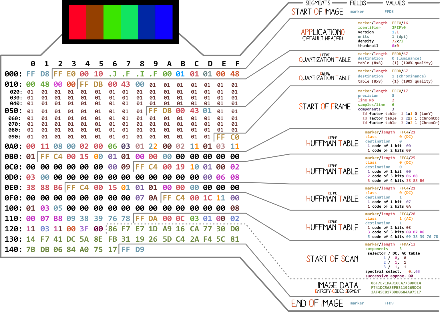
At the very basic level, almost every binary file contains a couple of markers (or headers). You can think of these markers as sort of like bookmarks. They are very crucial for making sense of a file and are used by programs like file (on Mac/Linux) to tell us details about a file. These markers define where some specific information in a file is stored. Most of the markers are followed by length information for the particular marker segment. This tells us how long that particular segment is.
File Start & File End
The very first marker we care about is FF D8. It tells us that this is the start of the image. If we don’t see it we can assume this is some other file. Another equally important marker is FF D9. It tells us that we have reached the end of an image file. Every marker, except for FFD0 to FFD9 and FF01, is immediately followed by a length specifier that will give you the length of that marker segment. As for the image file start and image file end markers, they will always be two bytes long each.
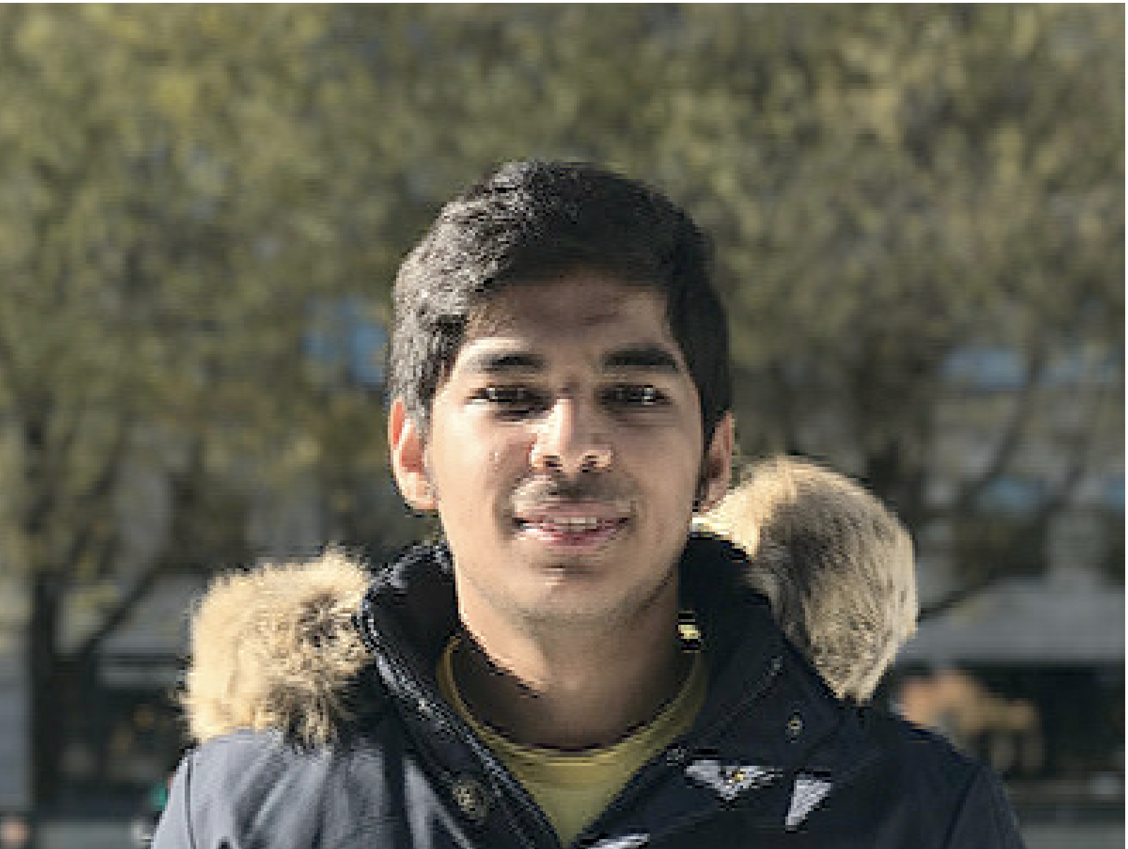
Throughout this tutorial, we will be working with this image:
Let’s write some code to identify these markers.
from struct import unpack


marker_mapping = {
    0xffd8: "Start of Image",
    0xffe0: "Application Default Header",
    0xffdb: "Quantization Table",
    0xffc0: "Start of Frame",
    0xffc4: "Define Huffman Table",
    0xffda: "Start of Scan",
    0xffd9: "End of Image"
}


class JPEG:
    def __init__(self, image_file):
        with open(image_file, 'rb') as f:
            self.img_data = f.read()

    def decode(self):
        data = self.img_data
        while(True):
            marker, = unpack(">H", data[0:2])
            print(marker_mapping.get(marker))
            if marker == 0xffd8:
                data = data[2:]
            elif marker == 0xffd9:
                return
            elif marker == 0xffda:
                data = data[-2:]
            else:
                lenchunk, = unpack(">H", data[2:4])
                data = data[2+lenchunk:]
            if len(data)==0:
                break

if __name__ == "__main__":
    img = JPEG('profile.jpg')
    img.decode()

# OUTPUT:
# Start of Image
# Application Default Header
# Quantization Table
# Quantization Table
# Start of Frame
# Huffman Table
# Huffman Table
# Huffman Table
# Huffman Table
# Start of Scan
# End of Image
We are using struct to unpack the bytes of image data. >H tells struct to treat the data as big-endian and of type unsigned short. The data in JPEG is stored in big-endian format. Only the EXIF data can be in little-endian (even though it is uncommon). And a short is of size 2 so we provide unpack two bytes from our img_data. You might ask yourself how we knew it was a short. Well, we know that the markers in JPEG are 4 hex digits: ffd8. One hex digit equals 4 bits (1/2 byte) so 4 hex digits will equal 2 bytes and a short is equal to 2 bytes.
The Start of Scan section is immediately followed by image scan data and that image scan data doesn’t have a length specified. It continues till the “end of file” marker is found so for now we are manually “seeking” to the EOF marker whenever we see the SOC marker.
Now that we have the basic framework in place, let’s move on and figure out what the rest of the image data contains. We will go through some necessary theory first and then get down to coding.
Encoding a JPEG
I will first explain some basic concepts and encoding techniques used by JPEG and then decoding will naturally follow from that as a reverse of it. In my experience, directly trying to make sense of decoding is a bit hard.
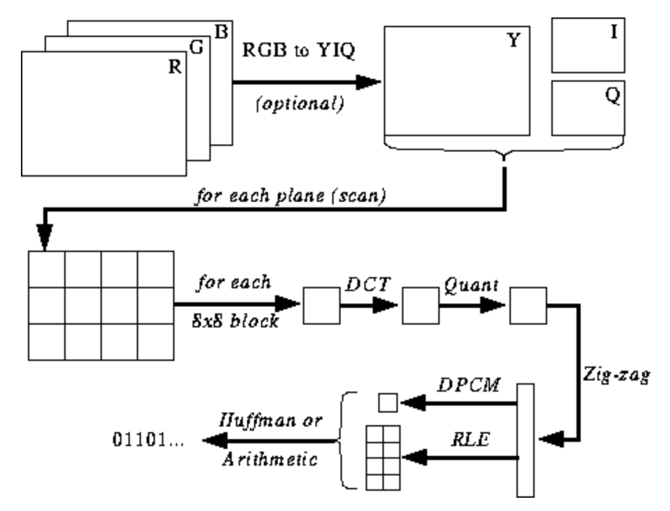
Even though the image below won’t mean much to you right now, it will give you some anchors to hold on to while we go through the whole encoding/decoding process. It shows the steps involved in the JPEG encoding process: (src)
JPEG Color Space
According to the JPEG spec (ISO/IEC 10918-6:2013 (E), section 6.1):
- Images encoded with only one component are assumed to be grayscale data in which 0 is black and 255 is white.
- Images encoded with three components are assumed to be RGB data encoded as YCbCr unless the image contains an APP14 marker segment as specified in 6.5.3, in which case the color encoding is considered either RGB or YCbCr according to the application data of the APP14 marker segment. The relationship between RGB and YCbCr is defined as specified in Rec. ITU-T T.871 | ISO/IEC 10918-5.
- Images encoded with four components are assumed to be CMYK, with (0,0,0,0) indicating white unless the image contains an APP14 marker segment as specified in 6.5.3, in which case the color encoding is considered either CMYK or YCCK according to the application data of the APP14 marker segment. The relationship between CMYK and YCCK is defined as specified in clause 7.
Most JPEG algorithm implementations use luminance and chrominance (YUV encoding) instead of RGB. This is super useful in JPEG as the human eye is pretty bad at seeing high-frequency brightness changes over a small area so we can essentially reduce the amount of frequency and the human eye won’t be able to tell the difference. Result? A highly compressed image with almost no visible reduction in quality.
Just like each pixel in RGB color space is made up of 3 bytes of color data (Red, Green, Blue), each pixel in YUV uses 3 bytes as well but what each byte represents is slightly different. The Y component determines the brightness of the color (also referred to as luminance or luma), while the U and V components determine the color (also known as chroma). The U component refers to the amount of blue color and the V component refers to the amount of red color.
This color format was invented when color televisions weren’t super common and engineers wanted to use one image encoding format for both color and black and white televisions. YUV could be safely displayed on a black and white TV if color wasn’t available. You can read more about its history on Wikipedia.
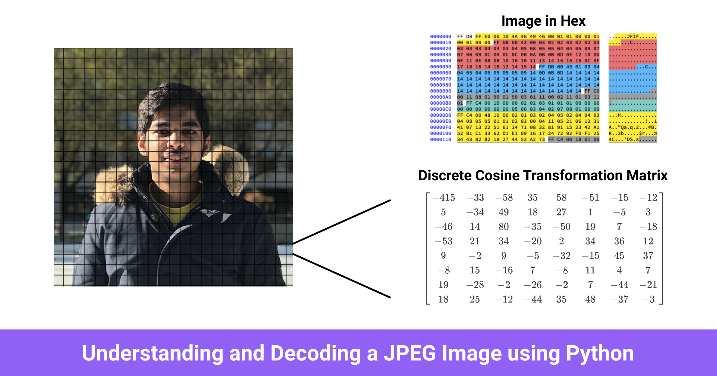
Discrete Cosine Transform & Quantization
JPEG converts an image into chunks of 8x8 blocks of pixels (called MCUs or Minimum Coding Units), changes the range of values of the pixels so that they center on 0 and then applies Discrete Cosine Transformation to each block and then uses quantization to compress the resulting block. Let’s get a high-level understanding of what all of these terms mean.
A Discrete Cosine Transform is a method for converting discrete data points into a combination of cosine waves. It seems pretty useless to spend time converting an image into a bunch of cosines but it makes sense once we understand DCT in combination with how the next step works. In JPEG, DCT will take an 8x8 image block and tell us how to reproduce it using an 8x8 matrix of cosine functions. Read more here)
The 8x8 matrix of cosine functions look like this:
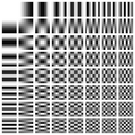
We apply DCT to each component of a pixel separately. The output of applying DCT is an 8x8 coefficient matrix that tells us how much each cosine function (out of 64 total functions) contributes to the 8x8 input matrix. The coefficient matrix of a DCT generally contains bigger values in the top left corner of the coefficient matrix and smaller values in the bottom right corner. The top left corner represents the lowest frequency cosine function and the bottom right represents the highest frequency cosine function.
What this tells us is that most images contain a huge amount of low-frequency information and a small amount of high-frequency information. If we turn the bottom right components of each DCT matrix to 0, the resulting image would still appear the same because, as I mentioned, humans are bad at observing high-frequency changes. This is exactly what we do in the next step.
I found a wonderful video on this topic. Watch it if DCT doesn’t make too much sense.
We have all heard that JPEG is a lossy compression algorithm but so far we haven’t done anything lossy. We have only transformed 8x8 blocks of YUV components into 8x8 blocks of cosine functions with no loss of information. The lossy part comes in the quantization step.
Quantization is a process in which we take a couple of values in a specific range and turns them into a discrete value. For our case, this is just a fancy name for converting the higher frequency coefficients in the DCT output matrix to 0. When you save an image using JPEG, most image editing programs ask you how much compression you need. The percentage you supply there affects how much quantization is applied and how much of higher frequency information is lost. This is where the lossy compression is applied. Once you lose high-frequency information, you can’t recreate the exact original image from the resulting JPEG image.
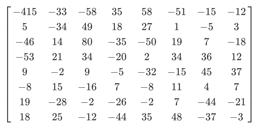
Depending on the compression level required, some common quantization matrices are used (fun fact: Most vendors have patents on quantization table construction). We divide the DCT coefficient matrix element-wise with the quantization matrix, round the result to an integer, and get the quantized matrix. Let’s go through an example.
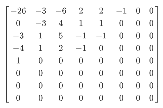
If you have this DCT matrix:
This (common) Quantization matrix:
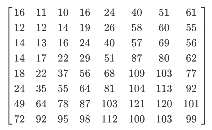
Then the resulting quantized matrix will be this:
Even though humans can’t see high-frequency information, if you remove too much information from the 8x8 image chunks, the overall image will look blocky. In this quantized matrix, the very first value is called a DC value and the rest of the values are AC values. If we were to take the DC values from all the quantized matrices and generated a new image, we will essentially end up with a thumbnail with 1/8th resolution of the original image.
It is also important to note that because we apply quantization while decoding, we will have to make sure the colors fall in the [0,255] range. If they fall outside this range, we will have to manually clamp them to this range.
Zig-zag
After quantization, JPEG uses zig-zag encoding to convert the matrix to 1D (img src):
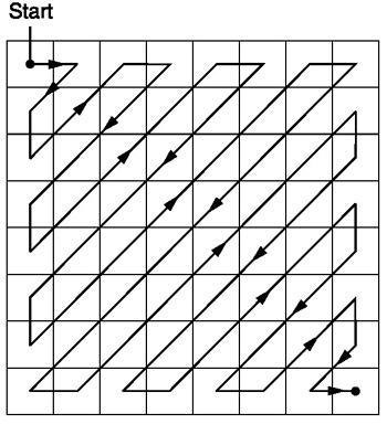
Let’s imagine we have this quantized matrix:
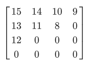
The output of zig-zag encoding will be this:
[15 14 13 12 11 10 9 8 0 ... 0]
This encoding is preferred because most of the low frequency (most significant) information is stored at the beginning of the matrix after quantization and the zig-zag encoding stores all of that at the beginning of the 1D matrix. This is useful for the compression that happens in the next step.
Run-length and Delta encoding
Run-length encoding is used to compress repeated data. At the end of the zig-zag encoding, we saw how most of the zig-zag encoded 1D arrays had so many 0s at the end. Run-length encoding allows us to reclaim all that wasted space and use fewer bytes to represent all of those 0s. Imagine you have some data like this:
10 10 10 10 10 10 10
Run-length encoding will convert it into:
7 10
We were able to successfully compress 7 bytes of data into only 2 bytes.
Delta encoding is a technique used to represent a byte relative to the byte before it. It is easier to understand this with an example. Let’s say you have the following data:
10 11 12 13 10 9
You can use delta encoding to store it like this:
10 1 2 3 0 -1
In JPEG, every DC value in a DCT coefficient matrix is delta encoded relative to the DC value preceding it. This means that if you change the very first DCT coefficient of your image, the whole image will get screwed up but if you modify the first value of the last DCT matrix, only a very tiny part of your image will be affected. This is useful because the first DC value in your image is usually the most varied and by applying the Delta encoding we bring the rest of DC values close to 0 and that results in better compression in the next step of Huffman Encoding.
Huffman Encoding
Huffman encoding is a method for lossless compression of information. Huffman once asked himself, “What’s the smallest number of bits I can use to store an arbitrary piece of text?”. This coding format was his answer. Imagine you have to store this text:
a b c d e
In a normal scenario each character would take up 1 byte of space:
a: 01100001
b: 01100010
c: 01100011
d: 01100100
e: 01100101
This is based on ASCII to binary mapping. But what if we could come up with a custom mapping?
# Mapping

000: 01100001
001: 01100010
010: 01100011
100: 01100100
011: 01100101
Now we can store the same text using way fewer bits:
a: 000
b: 001
c: 010
d: 100
e: 011
This is all well and good but what if we want to take even less space? What if we were able to do something like this:
# Mapping
0:  01100001
1:  01100010
00: 01100011
01: 01100100
10: 01100101

a: 0
b: 1
c: 00
d: 01
e: 10
Huffman encoding allows us to use this sort of variable-length mapping. It takes some input data, maps the most frequent characters to the smaller bit patterns and least frequent characters to larger bit patterns, and finally organizes the mapping into a binary tree. In a JPEG we store the DCT (Discrete Cosine Transform) information using Huffman encoding. Remember I told you that using delta encoding for DC values helps in Huffman Encoding? I hope you can see why now. After delta encoding, we end up with fewer “characters” to map and the total size of our Huffman tree is reduced.
Tom Scott has a wonderful video with animations on how Huffman encoding works in general. Do watch it before moving on.
A JPEG contains up to 4 Huffman tables and these are stored in the “Define Huffman Table” section (starting with 0xffc4). The DCT coefficients are stored in 2 different Huffman tables. One contains only the DC values from the zig-zag tables and the other contains the AC values from the zig-zag tables. This means that in our decoding, we will have to merge the DC and AC values from two separate matrices. The DCT information for the luminance and chrominance channel is stored separately so we have 2 sets of DC and 2 sets of AC information giving us a total of 4 Huffman tables.
In a greyscale image, we would have only 2 Huffman tables (1 for DC and 1 for AC) because we don’t care about the color. As you can already imagine, 2 images can have very different Huffman tables so it is important to store these tables inside each JPEG.
So we know the basic details of what a JPEG image contains. Let’s start with the decoding!
JPEG decoding
We can break down the decoding into a bunch of steps:
- Extract the Huffman tables and decode the bits
- Extract DCT coefficients by undoing the run-length and delta encodings
- Use DCT coefficients to combine cosine waves and regenerate pixel values for each 8x8 block
- Convert YCbCr to RGB for each pixel
- Display the resulting RGB image
JPEG standard supports 4 compression formats:
- Baseline
- Extended Sequential
- Progressive
- Lossless
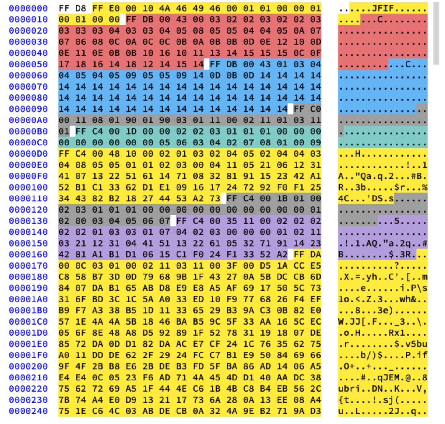
We are going to be working with the Baseline compression and according to the standard, baseline will contain the series of 8x8 blocks right next to each other. The other compression formats layout the data a bit differently. Just for reference, I have colored different segments in the hex content of the image we are using. This is how it looks:
Extracting the Huffman tables
We already know that a JPEG contains 4 Huffman tables. This is the last step in the encoding procedure so it should be the first step in the decoding procedure. Each DHT section contains the following information:
| Field | Size | Description |
|---|---|---|
| Marker Identifier | 2 bytes | 0xff, 0xc4 to identify DHT marker |
| Length | 2 bytes | This specifies the length of Huffman table |
| HT information | 1 byte | bit 0..3: number of HT (0..3, otherwise error) bit 4: type of HT, 0 = DC table, 1 = AC table bit 5..7: not used, must be 0 |
| Number of Symbols | 16 bytes | Number of symbols with codes of length 1..16, the sum(n) of these bytes is the total number of codes, which must be <= 256 |
| Symbols | n bytes | Table containing the symbols in order of increasing code length ( n = total number of codes ). |
Suppose you have a DH table similar to this (src):
| Symbol | Huffman code | Code length |
|---|---|---|
| a | 00 | 2 |
| b | 010 | 3 |
| c | 011 | 3 |
| d | 100 | 3 |
| e | 101 | 3 |
| f | 110 | 3 |
| g | 1110 | 4 |
| h | 11110 | 5 |
| i | 111110 | 6 |
| j | 1111110 | 7 |
| k | 11111110 | 8 |
| l | 111111110 | 9 |
It will be stored in the JFIF file roughly like this (they will be stored in binary. I am using ASCII just for illustration purposes):
0 1 5 1 1 1 1 1 1 0 0 0 0 0 0 0 a b c d e f g h i j k l
The 0 means that there is no Huffman code of length 1. 1 means that there is 1 Huffman code of length 2. And so on. There are always 16 bytes of length data in the DHT section right after the class and ID information. Let’s write some code to extract the lengths and elements in DHT.
class JPEG:
    # ...

    def decodeHuffman(self, data):
        offset = 0
        header, = unpack("B",data[offset:offset+1])
        offset += 1

        # Extract the 16 bytes containing length data
        lengths = unpack("BBBBBBBBBBBBBBBB", data[offset:offset+16])
        offset += 16

        # Extract the elements after the initial 16 bytes
        elements = []
        for i in lengths:
            elements += (unpack("B"*i, data[offset:offset+i]))
            offset += i

        print("Header: ",header)
        print("lengths: ", lengths)
        print("Elements: ", len(elements))
        data = data[offset:]


    def decode(self):
        data = self.img_data
        while(True):
            # ---
            else:
                len_chunk, = unpack(">H", data[2:4])
                len_chunk += 2
                chunk = data[4:len_chunk]

                if marker == 0xffc4:
                    self.decodeHuffman(chunk)
                data = data[len_chunk:]
            if len(data)==0:
                break
If you run the code, it should produce the following output:
Start of Image
Application Default Header
Quantization Table
Quantization Table
Start of Frame
Huffman Table
Header:  0
lengths:  (0, 2, 2, 3, 1, 1, 1, 0, 0, 0, 0, 0, 0, 0, 0, 0)
Elements:  10
Huffman Table
Header:  16
lengths:  (0, 2, 1, 3, 2, 4, 5, 2, 4, 4, 3, 4, 8, 5, 5, 1)
Elements:  53
Huffman Table
Header:  1
lengths:  (0, 2, 3, 1, 1, 1, 0, 0, 0, 0, 0, 0, 0, 0, 0, 0)
Elements:  8
Huffman Table
Header:  17
lengths:  (0, 2, 2, 2, 2, 2, 1, 3, 3, 1, 7, 4, 2, 3, 0, 0)
Elements:  34
Start of Scan
End of Image
Sweet! We got the lengths and the elements. Now we need to create a custom Huffman table class so that we can recreate a binary tree from these elements and lengths. I am shamelessly copying this code from here:
class HuffmanTable:
    def __init__(self):
        self.root=[]
        self.elements = []

    def BitsFromLengths(self, root, element, pos):
        if isinstance(root,list):
            if pos==0:
                if len(root)<2:
                    root.append(element)
                    return True
                return False
            for i in [0,1]:
                if len(root) == i:
                    root.append([])
                if self.BitsFromLengths(root[i], element, pos-1) == True:
                    return True
        return False

    def GetHuffmanBits(self,  lengths, elements):
        self.elements = elements
        ii = 0
        for i in range(len(lengths)):
            for j in range(lengths[i]):
                self.BitsFromLengths(self.root, elements[ii], i)
                ii+=1

    def Find(self,st):
        r = self.root
        while isinstance(r, list):
            r=r[st.GetBit()]
        return  r

    def GetCode(self, st):
        while(True):
            res = self.Find(st)
            if res == 0:
                return 0
            elif ( res != -1):
                return res

class JPEG:
    # -----

    def decodeHuffman(self, data):
        # ----
        hf = HuffmanTable()
        hf.GetHuffmanBits(lengths, elements)
        data = data[offset:]
The GetHuffmanBits takes in the lengths and elements, iterates over all the elements and puts them in a root list. This list contains nested lists and represents a binary tree. You can read online how a Huffman Tree works and how to create your own Huffman tree data structure in Python. For our first DHT (using the image I linked at the start of this tutorial) we have the following data, lengths, and elements:
Hex Data: 00 02 02 03 01 01 01 00 00 00 00 00 00 00 00 00
Lengths:  (0, 2, 2, 3, 1, 1, 1, 0, 0, 0, 0, 0, 0, 0, 0, 0)
Elements: [5, 6, 3, 4, 2, 7, 8, 1, 0, 9]
After calling GetHuffmanBits on this, the root list will contain this data:
[[5, 6], [[3, 4], [[2, 7], [8, [1, [0, [9]]]]]]]
The HuffmanTable also contains the GetCode method that traverses the tree for us and gives us back the decoded bits using the Huffman table. This method expects a bitstream as an input. A bitstream is just the binary representation of data. For example, a typical bitstream of abc will be 011000010110001001100011. We first convert each character into its ASCII code and then convert that ASCII code to binary. Let’s create a custom class that will allow us to convert a string into bits and read the bits one by one. This is how we will implement it:
class Stream:
    def __init__(self, data):
        self.data= data
        self.pos = 0

    def GetBit(self):
        b = self.data[self.pos >> 3]
        s = 7-(self.pos & 0x7)
        self.pos+=1
        return (b >> s) & 1

    def GetBitN(self, l):
        val = 0
        for i in range(l):
            val = val*2 + self.GetBit()
        return val
We feed this class some binary data while initializing it and then use the GetBit and GetBitN methods to read it.
Decoding the Quantization Table
The Define Quantization Table section contains the following data:
| Field | Size | Description |
|---|---|---|
| Marker Identifier | 2 bytes | 0xff, 0xdb identifies DQT |
| Length | 2 bytes | This gives the length of QT. |
| QT information | 1 byte | bit 0..3: number of QT (0..3, otherwise error) bit 4..7: the precision of QT, 0 = 8 bit, otherwise 16 bit |
| Bytes | n bytes | This gives QT values, n = 64*(precision+1) |
According to the JPEG standard, there are 2 default quantization tables in a JPEG image. One for luminance and one for chrominance. These tables start at the 0xffdb marker. In the initial code we wrote, we already saw that the output contained two 0xffdb markers. Let’s extend the code we already have and add the ability to decode quantization tables as well:
def GetArray(type,l, length):
    s = ""
    for i in range(length):
        s =s+type
    return list(unpack(s,l[:length]))

class JPEG:
    # ------
    def __init__(self, image_file):
        self.huffman_tables = {}
        self.quant = {}
        with open(image_file, 'rb') as f:
            self.img_data = f.read()

    def DefineQuantizationTables(self, data):
        hdr, = unpack("B",data[0:1])
        self.quant[hdr] =  GetArray("B", data[1:1+64],64)
        data = data[65:]


    def decodeHuffman(self, data):
        # ------
        for i in lengths:
            elements += (GetArray("B", data[off:off+i], i))
            offset += i
            # ------

    def decode(self):
        # ------
        while(True):
            # ----
            else:
                # -----
                if marker == 0xffc4:
                    self.decodeHuffman(chunk)
                elif marker == 0xffdb:
                    self.DefineQuantizationTables(chunk)
                data = data[len_chunk:]
            if len(data)==0:
                break
We did a couple of things here. First, I defined a GetArray method. It is just a handy method for decoding a variable number of bytes from binary data. I replaced some code in decodeHuffman method to make use of this new function as well. After that, I defined the DefineQuantizationTables method. This method simply reads the header of a Quantization Table section and then appends the quantization data in a dictionary with the header value as the key. The header value will be 0 for luminance and 1 for chrominance. Each Quantization Table section in the JFIF contains 64 bytes of QT data (for our 8x8 Quantization matrix).
If we print the quantization matrices for our image. They will look like this:
3    2    2    3    2    2    3    3
3    3    4    3    3    4    5    8
5    5    4    4    5    10   7    7
6    8    12   10   12   12   11   10
11   11   13   14   18   16   13   14
17   14   11   11   16   22   16   17
19   20   21   21   21   12   15   23
24   22   20   24   18   20   21   20


3     2    2    3    2    2    3    3
3     2    2    3    2    2    3    3
3     3    4    3    3    4    5    8
5     5    4    4    5    10   7    7
6     8    12   10   12   12   11   10
11    11   13   14   18   16   13   14
17    14   11   11   16   22   16   17
19    20   21   21   21   12   15   23
24    22   20   24   18   20   21   20
Decoding Start of Frame
The Start of Frame section contains the following information (src):
| Field | Size | Description |
|---|---|---|
| Marker Identifier | 2 bytes | 0xff, 0xc0 to identify SOF0 marker |
| Length | 2 bytes | This value equals to 8 + components*3 value |
| Data precision | 1 byte | This is in bits/sample, usually 8 (12 and 16 not supported by most software). |
| Image height | 2 bytes | This must be > 0 |
| Image Width | 2 bytes | This must be > 0 |
| Number of components | 1 byte | Usually 1 = grey scaled, 3 = color YcbCr or YIQ |
| Each component | 3 bytes | Read each component data of 3 bytes. It contains, (component Id(1byte)(1 = Y, 2 = Cb, 3 = Cr, 4 = I, 5 = Q), sampling factors (1byte) (bit 0-3 vertical., 4-7 horizontal.), quantization table number (1 byte)). |
Out of this data we only care about a few things. We will extract the image width and height and the quantization table number of each component. The width and height will be used when we start decoding the actual image scans from the Start of Scan section. Because we are going to be mainly working with a YCbCr image, we can expect the number of components to be equal to 3 and the component types to be equal to 1, 2 and 3 respectively. Let’s write some code to decode this data:
class JPEG:
    def __init__(self, image_file):
        self.huffman_tables = {}
        self.quant = {}
        self.quantMapping = []
        with open(image_file, 'rb') as f:
            self.img_data = f.read()
    # ----
    def BaselineDCT(self, data):
        hdr, self.height, self.width, components = unpack(">BHHB",data[0:6])
        print("size %ix%i" % (self.width,  self.height))

        for i in range(components):
            id, samp, QtbId = unpack("BBB",data[6+i*3:9+i*3])
            self.quantMapping.append(QtbId)

    def decode(self):
        # ----
        while(True):
                # -----
                elif marker == 0xffdb:
                    self.DefineQuantizationTables(chunk)
                elif marker == 0xffc0:
                    self.BaselineDCT(chunk)
                data = data[len_chunk:]
            if len(data)==0:
                break
We added a quantMapping list attribute to our JPEG class and introduced a BaselineDCT method. The BaselineDCT method decodes the required data from the SOF section and puts the quantization table numbers of each component in the quantMapping list. We will make use of this mapping once we start reading the Start of Scan section. This is what the quantMapping looks like for our image:
Quant mapping: [0, 1, 1]
Decoding Start of Scan
Sweet! We only have one more section left to decode. This is the meat of a JPEG image and contains the actual “image” data. This is also the most involved step. Everything else we have decoded so far can be thought of as creating a map to help us navigate and decode the actual image. This section contains the actual image itself (albeit in an encoded form). We will read this section and use the data we have already decoded to make sense of the image.
All the markers we have seen so far start with 0xff. 0xff can be part of the image scan data as well but if 0xff is present in the scan data, it will always be proceeded by 0x00. This is something a JPEG encoder does automatically and is called byte stuffing. It is the decoder’s duty to remove this proceeding 0x00. Let’s start the SOS decoder method with this function and get rid of 0x00 if it is present. In the sample image I am using, we don’t have 0xff in the image scan data but it is nevertheless a useful addition.
def RemoveFF00(data):
    datapro = []
    i = 0
    while(True):
        b,bnext = unpack("BB",data[i:i+2])
        if (b == 0xff):
            if (bnext != 0):
                break
            datapro.append(data[i])
            i+=2
        else:
            datapro.append(data[i])
            i+=1
    return datapro,i

class JPEG:
    # ----
    def StartOfScan(self, data, hdrlen):
        data,lenchunk = RemoveFF00(data[hdrlen:])
        return lenchunk+hdrlen

    def decode(self):
        data = self.img_data
        while(True):
            marker, = unpack(">H", data[0:2])
            print(marker_mapping.get(marker))
            if marker == 0xffd8:
                data = data[2:]
            elif marker == 0xffd9:
                return
            else:
                len_chunk, = unpack(">H", data[2:4])
                len_chunk += 2
                chunk = data[4:len_chunk]
                if marker == 0xffc4:
                    self.decodeHuffman(chunk)
                elif marker == 0xffdb:
                    self.DefineQuantizationTables(chunk)
                elif marker == 0xffc0:
                    self.BaselineDCT(chunk)
                elif marker == 0xffda:
                    len_chunk = self.StartOfScan(data, len_chunk)
                data = data[len_chunk:]
            if len(data)==0:
                break
Previously I was manually seeking to the end of the file whenever I encountered the 0xffda marker but now that we have the required tooling in place to go through the whole file in a systematic order, I moved the marker condition inside the else clause. The RemoveFF00 function simply breaks whenever it observer something other than 0x00 after 0xff. Therefore, it will break out of the loop when it encounters 0xffd9, and that way we can safely seek to the end of the file without any surprises. If you run this code now, nothing new will output to the terminal.
Recall that JPEG broke up the image into an 8x8 matrix. The next step for us is to convert our image scan data into a bit-stream and process the stream in 8x8 chunks of data. Let’s add some more code to our class:
class JPEG:
    # -----
    def StartOfScan(self, data, hdrlen):
        data,lenchunk = RemoveFF00(data[hdrlen:])
        st = Stream(data)
        oldlumdccoeff, oldCbdccoeff, oldCrdccoeff = 0, 0, 0
        for y in range(self.height//8):
            for x in range(self.width//8):
                matL, oldlumdccoeff = self.BuildMatrix(st,0, self.quant[self.quantMapping[0]], oldlumdccoeff)
                matCr, oldCrdccoeff = self.BuildMatrix(st,1, self.quant[self.quantMapping[1]], oldCrdccoeff)
                matCb, oldCbdccoeff = self.BuildMatrix(st,1, self.quant[self.quantMapping[2]], oldCbdccoeff)
                DrawMatrix(x, y, matL.base, matCb.base, matCr.base )

        return lenchunk +hdrlen
We start by converting our scan data into a bit-stream. Then we initialize oldlumdccoeff, oldCbdccoeff, oldCrdccoeff to 0. These are required because remember we talked about how the DC element in a quantization matrix (the first element of the matrix) is delta encoded relative to the previous DC element? This will help us keep track of the value of the previous DC elements and 0 will be the default when we encounter the first DC element.
The for loop might seem a bit funky. The self.height//8 tells us how many times we can divide the height by 8. The same goes for self.width//8. This in short tells us how many 8x8 matrices is the image divided in.
The BuildMatrix will take in the quantization table and some additional params, create an Inverse Discrete Cosine Transformation Matrix, and give us the Y, Cr, and Cb matrices. The actual conversion of these matrices to RGB will happen in the DrawMatrix function.
Let’s first create our IDCT class and then we can start fleshing out the BuildMatrix method.
import math


class IDCT:
    """
    An inverse Discrete Cosine Transformation Class
    """

    def __init__(self):
        self.base = [0] * 64
        self.zigzag = [
            [0, 1, 5, 6, 14, 15, 27, 28],
            [2, 4, 7, 13, 16, 26, 29, 42],
            [3, 8, 12, 17, 25, 30, 41, 43],
            [9, 11, 18, 24, 31, 40, 44, 53],
            [10, 19, 23, 32, 39, 45, 52, 54],
            [20, 22, 33, 38, 46, 51, 55, 60],
            [21, 34, 37, 47, 50, 56, 59, 61],
            [35, 36, 48, 49, 57, 58, 62, 63],
        ]
        self.idct_precision = 8
        self.idct_table = [
            [
                (self.NormCoeff(u) * math.cos(((2.0 * x + 1.0) * u * math.pi) / 16.0))
                for x in range(self.idct_precision)
            ]
            for u in range(self.idct_precision)
        ]

    def NormCoeff(self, n):
        if n == 0:
            return 1.0 / math.sqrt(2.0)
        else:
            return 1.0

    def rearrange_using_zigzag(self):
        for x in range(8):
            for y in range(8):
                self.zigzag[x][y] = self.base[self.zigzag[x][y]]
        return self.zigzag

    def perform_IDCT(self):
        out = [list(range(8)) for i in range(8)]

        for x in range(8):
            for y in range(8):
                local_sum = 0
                for u in range(self.idct_precision):
                    for v in range(self.idct_precision):
                        local_sum += (
                            self.zigzag[v][u]
                            * self.idct_table[u][x]
                            * self.idct_table[v][y]
                        )
                out[y][x] = local_sum // 4
        self.base = out
Let’s try to understand this IDCT class step by step. Once we extract the MCU from a JPEG, the base attribute of this class will store it. Then we will rearrange the MCU matrix by undoing the zigzag encoding via the rearrange_using_zigzag method. Finally, we will undo the Discrete Cosine Transformation by calling the perform_IDCT method.
If you remember, the Discrete Cosine table is fixed. How the actual calculation for a DCT works is outside the scope of this tutorial as it is more maths than programming. We can store this table as a global variable and then query that for values based on x,y pairs. I decided to put the table and its calculation in the IDCT class for readability purposes. Every single element of the rearranged MCU matrix is multiplied by the values of the idc_variable and we eventually get back the Y, Cr, and Cb values.
This will make more sense once we write down the BuildMatrix method.
If you modify the zigzag table to something like this:
[[ 0,  1,  5,  6, 14, 15, 27, 28],
[ 2,  4,  7, 13, 16, 26, 29, 42],
[ 3,  8, 12, 17, 25, 30, 41, 43],
[20, 22, 33, 38, 46, 51, 55, 60],
[21, 34, 37, 47, 50, 56, 59, 61],
[35, 36, 48, 49, 57, 58, 62, 63],
[ 9, 11, 18, 24, 31, 40, 44, 53],
[10, 19, 23, 32, 39, 45, 52, 54]]
You will have the following output (notice the small artifacts):
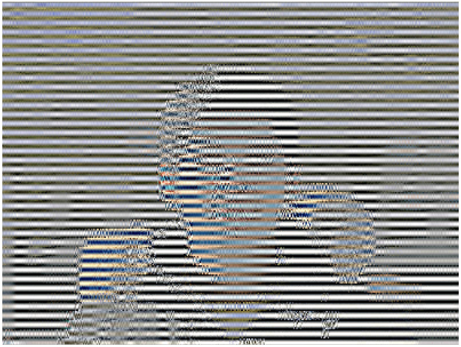
And if you are even brave, you can modify the zigzag table even more:
[[12, 19, 26, 33, 40, 48, 41, 34,],
[27, 20, 13,  6,  7, 14, 21, 28,],
[ 0,  1,  8, 16,  9,  2,  3, 10,],
[17, 24, 32, 25, 18, 11,  4,  5,],
[35, 42, 49, 56, 57, 50, 43, 36,],
[29, 22, 15, 23, 30, 37, 44, 51,],
[58, 59, 52, 45, 38, 31, 39, 46,],
[53, 60, 61, 54, 47, 55, 62, 63]]
It will result in this output:
Now let’s finish up our BuildMatrix method:
def DecodeNumber(code, bits):
    l = 2**(code-1)
    if bits>=l:
        return bits
    else:
        return bits-(2*l-1)


class JPEG:
    # -----
    def BuildMatrix(self, st, idx, quant, olddccoeff):
        i = IDCT()

        code = self.huffman_tables[0 + idx].GetCode(st)
        bits = st.GetBitN(code)
        dccoeff = DecodeNumber(code, bits) + olddccoeff

        i.base[0] = (dccoeff) * quant[0]
        l = 1
        while l < 64:
            code = self.huffman_tables[16 + idx].GetCode(st)
            if code == 0:
                break

            # The first part of the AC quantization table
            # is the number of leading zeros
            if code > 15:
                l += code >> 4
                code = code & 0x0F

            bits = st.GetBitN(code)

            if l < 64:
                coeff = DecodeNumber(code, bits)
                i.base[l] = coeff * quant[l]
                l += 1

        i.rearrange_using_zigzag()
        i.perform_IDCT()

        return i, dccoeff
We start by creating an Inverse Discrete Cosine Transformation class (IDCT()). Then we read in the bit-stream and decode it using our Huffman table.
The self.huffman_tables[0] and self.huffman_tables[1] refer to the DC tables for luminance and chrominance respectively and self.huffman_tables[16] and self.huffman_tables[17] refer to the AC tables for luminance and chrominance respectively.
After we decode the bit-stream, we extract the new delta encoded DC coefficient using the DecodeNumber function and add the olddccoefficient to it to get the delta decoded DC coefficient.
After that, we repeat the same decoding procedure but for the AC values in the quantization matrix. The code value of 0 suggests that we have encountered an End of Block (EOB) marker and we need to stop. Moreover, the first part of the AC quant table tells us how many leading 0’s we have. Remember the run-length encoding we talked about in the first part? This is where that is coming into play. We decode the run-length encoding and skip forward that many bits. The skipped bits are all set to 0 implicitly in the IDCT class.
Once we have decoded the DC and AC values for an MCU, we rearrange the MCU and undo the zigzag encoding by calling the rearrange_using_zigzag and then we perform inverse DCT on the decoded MCU.
The BuildMatrix method will return the inverse DCT matrix and the value of the DC coefficient. Remember, this inverse DCT matrix is only for one tiny 8x8 MCU (Minimum Coded Unit) matrix. We will be doing this for all the individual MCUs in the whole image file.
Displaying Image on screen
Let’s modify our code a little bit and create a Tkinter Canvas and paint each MCU after decoding it in the StartOfScan method.
def Clamp(col):
    col = 255 if col>255 else col
    col = 0 if col<0 else col
    return  int(col)

def ColorConversion(Y, Cr, Cb):
    R = Cr*(2-2*.299) + Y
    B = Cb*(2-2*.114) + Y
    G = (Y - .114*B - .299*R)/.587
    return (Clamp(R+128),Clamp(G+128),Clamp(B+128) )

def DrawMatrix(x, y, matL, matCb, matCr):
    for yy in range(8):
        for xx in range(8):
            c = "#%02x%02x%02x" % ColorConversion(
                matL[yy][xx], matCb[yy][xx], matCr[yy][xx]
            )
            x1, y1 = (x * 8 + xx) * 2, (y * 8 + yy) * 2
            x2, y2 = (x * 8 + (xx + 1)) * 2, (y * 8 + (yy + 1)) * 2
            w.create_rectangle(x1, y1, x2, y2, fill=c, outline=c)


class JPEG:
    # -----
    def StartOfScan(self, data, hdrlen):
        data,lenchunk = RemoveFF00(data[hdrlen:])
        st = Stream(data)
        oldlumdccoeff, oldCbdccoeff, oldCrdccoeff = 0, 0, 0
        for y in range(self.height//8):
            for x in range(self.width//8):
                matL, oldlumdccoeff = self.BuildMatrix(st,0, self.quant[self.quantMapping[0]], oldlumdccoeff)
                matCr, oldCrdccoeff = self.BuildMatrix(st,1, self.quant[self.quantMapping[1]], oldCrdccoeff)
                matCb, oldCbdccoeff = self.BuildMatrix(st,1, self.quant[self.quantMapping[2]], oldCbdccoeff)
                DrawMatrix(x, y, matL.base, matCb.base, matCr.base )

        return lenchunk+hdrlen


if __name__ == "__main__":
    from tkinter import *
    master = Tk()
    w = Canvas(master, width=1600, height=600)
    w.pack()
    img = JPEG('profile.jpg')
    img.decode()
    mainloop()
Let’s start with the ColorConversion and Clamp functions. ColorConversion takes in the Y, Cr, and Cb values, uses a formula to convert these values to their RGB counterparts, and then outputs the clamped RGB values. You might wonder why we are adding 128 to the RGB values. If you remember, before JPEG compressor applies DCT on the MCU, it subtracts 128 from the color values. If the colors were originally in the range [0,255], JPEG puts them into [-128,+128] range. So we have to undo that effect when we decode the JPEG and that is why we are adding 128 to RGB. As for the Clamp, during the decompression, the output value might exceed [0,255] so we clamp them between [0,255] .
In the DrawMatrix method, we loop over each 8x8 decoded Y, Cr, and Cb matrices and convert each element of the 8x8 matrices into RGB values. After conversion, we draw each pixel on the Tkinter canvas using the create_rectangle method. You can find the complete code on GitHub. Now if you run this code, my face will show up on your screen 😄
Conclusion
Oh boy! Who would have thought it would take 6000 word+ explanation for showing my face on the screen. I am amazed by how smart some of these algorithm inventors are! I hope you enjoyed this article as much as I enjoyed writing it. I learned a ton while writing this decoder. I never realized how much fancy math goes into the encoding of a simple JPEG image. I might work on a PNG image next and try writing a decoder for a PNG image. You should also try to write a decoder for a PNG (or some other format). I am sure it will involve a lot of learning and even more hex fun 😅
Either way, I am tired now. I have been staring at hex for far too long and I think I have earned a well-deserved break. You all take care and if you have any questions please write them in the comments below. I am super new to this JPEG coding adventure but I will try to answer as much as I possibly can 😄
Bye! 👋 ❤️
Further reading
If you want to delve into more detail, you can take a look at a few resource I used while writing this article. I have also added some additional links for some interesting JPEG related stuff:
- An illustrated guide to Unraveling the JPEG
- An extremely detailed article on JPEG Huffman Coding
- Let’s write a simple JPEG library. Uses C++
- Python 3 struct documentation
- Read this article on how FB used this knowledge about JPEG
- JPEG File layout and format
- An interesting presentation by Department of Defense on JPEG forensics
judge_c123c1c1
Firoze Sethna
Henning
Yasoob
In reply to Henning
John
Yasoob
In reply to John
Alvin
kristoff
Mohamad Saeed Gh
Kristoff Bonne
In reply to Mohamad Saeed Gh
Markus
MyName
Jonah
dan